Fishnets and overlapping polygons
Today a question was asked in the geocompr discord. I wanted to share part of the solution as I think it covers 2 helpful things:
- making a fishnet grid
- calculating the area of overlap between two polygons
For this example I’m using data from the Atlanta GIS Open Data Portal. Specifically using the future land use polygons.
I’ve downloaded a local copy of the data as a geojson. But you can read it using the ArcGIS Feature Server it is hosted on.
Objective
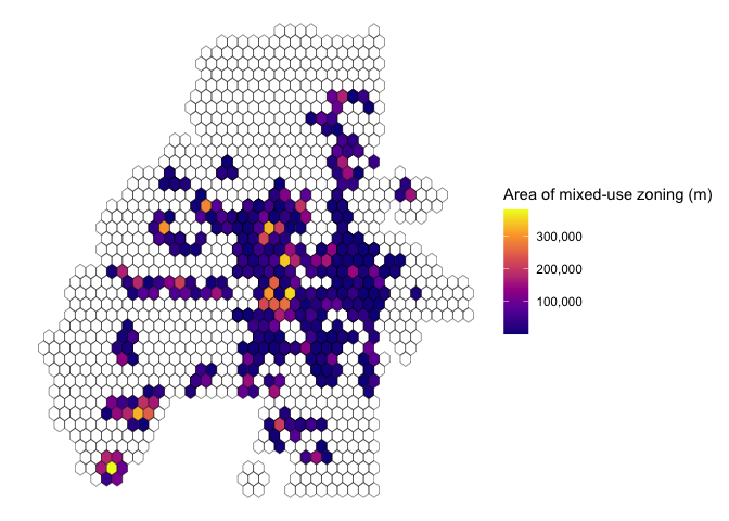
Create a map of Atlanta, visualized as a hexagon grid, that displays the amount of planned mixed use zoning. This will be done in the following sequence:
- Creating a fishnet (hexagon) grid over the city
- Creating intersected polygons
- Calculate the area of intersected polygons
- Join back to the original fishnet grid
- visualized.
Mixed-use zoning
Start by loading sf, dplyr, and ggplot2. sf for our spatial work, dplyr for making our lives easier, and ggplot2 for a bad map later.
We read in our data (mine is local). You can use the commented out code to read directly from the ArcGIS feature server.
# read from the ArcGIS feature server
# st_read("https://services5.arcgis.com/5RxyIIJ9boPdptdo/arcgis/rest/services/Land_Use_Future/FeatureServer/0/query?outFields=*&where=1%3D1&f=geojson")
future_land_use <- |>
Let’s look at the different land use descriptions.
future_land_use |>
|>
|>
reactable::
To see a disgusting map with a bad legend run the following.
future_land_use |>
+
We can see that there are a bunch of different descriptions for
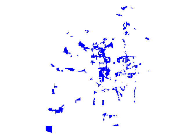
different types of mixed use zoning. Let’s filter down to descriptions
that have "Mixed-Use" or "Mixed Use" and visualize them.
# how much area of mixed use land use?
mixed_use <- future_land_use |>
+
+
Making a fishnet grid
Having made a fishnet grid quite a few times, I’ve got this handy function. In essence we create a grid over our target geometry and we keep only those locations from the grid that intersect eachother. If we dont’, we have a square shaped grid.
It is important that you create an ID for the grid, otherwise when we intersect later you’ll not know what is being intersected.
{
g <-
g
}
grd <- |>
|>
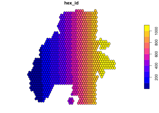
Man, I love maps of sequential IDs.
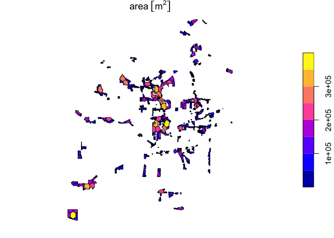
Next, we split our mixed use polygons based on the hexagons.
# how much area in each hexagon
lu_intersects <-
Warning: attribute variables are assumed to be spatially constant throughout
all geometries
Then we calculate the area of each resultant shape.
overlap_area <- lu_intersects |>
The next step here is to take the split polygons, and join the data back to the hexagons. I use a right join because they don’t get enough love. And also because if you try to do a join with two sf objects they’ll scream!!.
# join it back to the grid
hex_area_overlap <- |>
|>
|>
hex_area_overlap
Simple feature collection with 1381 features and 2 fields
Geometry type: POLYGON
Dimension:     XY
Bounding box:  xmin: -84.55738 ymin: 33.64417 xmax: -84.28635 ymax: 33.88926
Geodetic CRS:  WGS 84
# A tibble: 1,381 × 3
   hex_id    area                                                              x
    <int>   [m^2]                                                  <POLYGON [°]>
 1     72 160485. ((-84.5182 33.65548, -84.52146 33.65737, -84.52146 33.66114, …
 2     84  44538. ((-84.51493 33.64983, -84.5182 33.65171, -84.5182 33.65548, -…
 3     85 176134. ((-84.51493 33.66114, -84.5182 33.66302, -84.5182 33.66679, -…
 4     87   5049. ((-84.51493 33.68376, -84.5182 33.68565, -84.5182 33.68942, -…
 5     97 380145. ((-84.51167 33.65548, -84.51493 33.65737, -84.51493 33.66114,…
 6    100 110821. ((-84.51167 33.68942, -84.51493 33.6913, -84.51493 33.69507, …
 7    106   8232. ((-84.51167 33.75729, -84.51493 33.75917, -84.51493 33.76294,…
 8    110 109249. ((-84.5084 33.64983, -84.51167 33.65171, -84.51167 33.65548, …
 9    111 150687. ((-84.5084 33.66114, -84.51167 33.66302, -84.51167 33.66679, …
10    113 141654. ((-84.5084 33.68376, -84.51167 33.68565, -84.51167 33.68942, …
# ℹ 1,371 more rows
Now plot it!
+
+
+
+